Analyzing Particle Data with yt
Note: The dependencies for the yt analysis tools are not installed by default. You can install them with opencosmo install haloviz.
yt is an open-source Python package for analyzing and visualizing volumetric simulation data. Although yt was originally designed with AMR (Adaptive Mesh Refinement) codes in mind, support for SPH (Smoothed Particle Hydrodynamics) data is continually improving. As of yt version 4.4, most core functionality works reliably with SPH data, though some features may still require workarounds. In many cases, this involves depositing particle data onto a mesh using a YTArbitraryGrid object before passing it to specific yt functions.
In OpenCosmo, you can load particle datasets into yt using opencosmo.analysis.create_yt_dataset().
This is effectly doing the same as yt.load, however, we have opted to use the OpenCosmo toolkit
to handle the initial data selection.
Here is an example for how to use create_yt_dataset to load a selection of data into yt and make a simple projection
from opencosmo.analysis import create_yt_dataset, ParticleProjectionPlot

# select a random halo
with oc.open("haloproperties.hdf5", "haloparticles.hdf5").take(1, at="random") as data:
    # get yt data container
    yt_ds = create_yt_dataset(next(data.halos()))

    # list all fields
    print(yt_ds.derived_field_list)

    # project DM particle mass
    ParticleProjectionPlot(yt_ds, "z", ("dm", "particle_mass")).save()
For convenience, OpenCosmo includes wrappers for several commonly used yt plotting functions, including:
opencosmo.analysis.ParticleProjectionPlot()(wrapsyt.ParticleProjectionPlot)opencosmo.analysis.ProjectionPlot()(wrapsyt.ProjectionPlot)opencosmo.analysis.SlicePlot()(wrapsyt.SlicePlot)opencosmo.analysis.ProfilePlot()(wrapsyt.ProfilePlot)opencosmo.analysis.PhasePlot()(wrapsyt.PhasePlot)
These wrappers follow the same naming conventions as the original yt functions and have been verified to work out-of-the-box with HACC SPH data.
For an overview of yt’s broader functionality, refer to the official yt documentation.
For introductory tutorials, see:
Simulating X-ray Emission with pyXSIM
To include synthetic X-ray emissivity and luminosity fields from gas particles in your yt dataset, you can enable the compute_xray_fields flag when calling opencosmo.analysis.create_yt_dataset(). This integrates with pyXSIM, a toolkit for generating synthetic X-ray observations from simulation data.
When compute_xray_fields=True, the function internally creates a pyxsim.CIESourceModel using the particle data and attaches the following derived fields to the yt dataset:
X-ray emissivity per particle
X-ray luminosity in a user-specified energy band
Any additional fields required for photon sampling (e.g., emission measure)
You can also pass model-specific configurations via the source_model_kwargs argument, which is forwarded directly to the pyxsim.CIESourceModel constructor. Common options include:
emin(float): Minimum photon energy in keV (default: 0.1)emax(float): Maximum photon energy in keV (default: 10.0)nbins(int): Number of bins across the energy band (default: 1000)model(str): which emission model to use (default: “apec”)
For the full list of options, see CIESourceModel.
If return_source_model=True, the function will return a 2-tuple (ds, source_model), where source_model is the CIESourceModel instance. This allows further customization or photon generation using pyXSIM directly.
We will now edit the code-block from before to compute X-ray luminosities:
from opencosmo.analysis import create_yt_dataset, ParticleProjectionPlot

# set source model parameters
source_model_kwargs = {
    "emin": 0.1, # keV
    "emax": 10.0 # keV
}

# select a random halo
with oc.open("haloproperties.hdf5", "haloparticles.hdf5").take(1, at="random") as data:
    # get yt data container
    ds_yt, source_model = create_yt_dataset(next(data.halos()),
        compute_xray_fields = True, return_source_model = True)

    # list all fields
    print(ds_yt.derived_field_list)

    # project X-ray luminosity in the specified band
    ParticleProjectionPlot(ds_yt, "z", ("gas", "xray_luminosity_0.1_10.0_keV")).save()
Visualizing Halos
In addition to individual yt plots, OpenCosmo provides utilities for visualizing multiple halo projections at once.
The two primary functions for this purpose are:
opencosmo.analysis.visualize_halo()— a simple 2x2 panel plot for one haloopencosmo.analysis.halo_projection_array()— a customizable grid of halos and fields
These use yt under the hood, and are useful for visually inspecting halos with minimal input required. Animated versions of the visualizations outputted by either of these functions can be made using opencosmo.analysis.animate_halos().
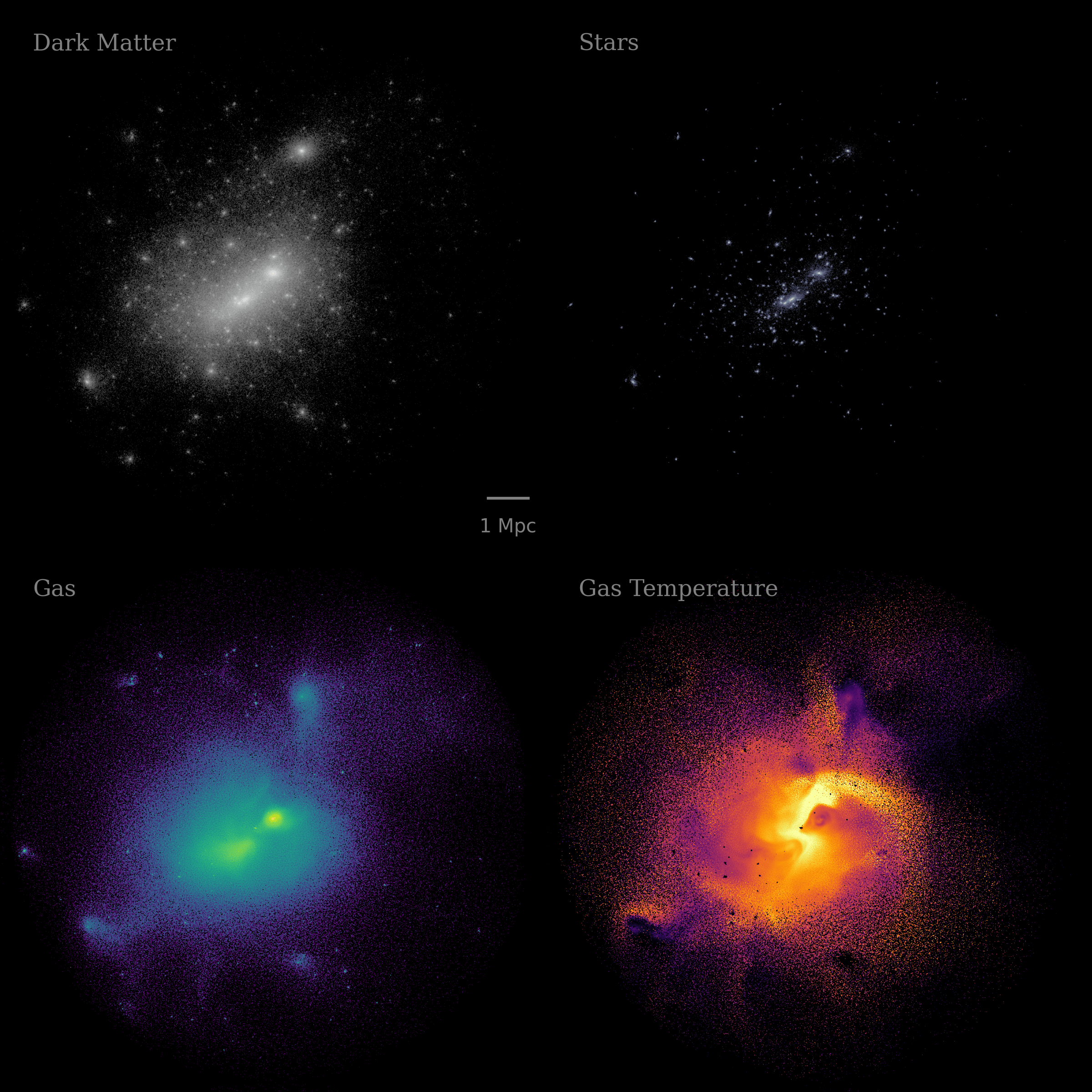
Quick Projections
The visualize_halo() function takes in a single halo ID and creates a multi-panel image showing particle projections of dark matter, stars, gas, and/or gas temperature for a the halo. If "dm"/"gravity", "star", and "gas" particles are all present, this will output a 2x2-panel figure. Otherwise, this will create a 1xN-panel figure showing whichever particles/fields from the list are present.
This function essentially uses halo_projection_array() with pre-filled settings for fields, colormaps, and labels.
Settings are tuned to look good for halos with \(M_\mathrm{200c} > 10^{14}\ M_\odot\).
from opencosmo.analysis import visualize_halo
import opencosmo as oc
import matplotlib.pyplot as plt

# load one halo at random
with oc.open("haloproperties.hdf5", "haloparticles.hdf5").take(1, at="random") as data:
    halo = next(data.halos())
    halo_id = halo["halo_properties"]["unique_tag"]

    fig = visualize_halo(halo_id, data)

# save the image
fig.savefig("halo_2x2_example.png")
A More Customizable Option
The halo_projection_array() function allows fine-grained control over what gets visualized, including:
Plotting different halos and/or fields per panel
Weighting projections by other quantities
Using different colormaps and colorbar limits
Customizing panel labels and layout
For the full list of customization options, see opencosmo.analysis.halo_projection_array()
Multiple Halos, Single Field
At minimum, halo_projection_array() takes in a 2D array of halo IDs and the StructuredCollection dataset containing the relevant halos.
The outputted figure is an array of images, with the shape matching that of the halo ID array. For example:
from opencosmo.analysis import halo_projection_array
import opencosmo as oc
import matplotlib.pyplot as plt
import numpy as np

# load 16 halos at random
with oc.open("haloproperties.hdf5", "haloparticles.hdf5").take(16, at="random") as data:

    halo_ids = [halo['halo_properties']['unique_tag'] for halo in data.halos()]

    # construct 4x4 array of halo ids and make a 4x4 array of dark matter projections
    fig = halo_projection_array(np.reshape(halo_ids,(4,4)), data,
                field=("dm","particle_mass"), width=6.0)

# save the image
fig.savefig("halo_4x4_example.png")

Multiple Halos, Multiple Fields
One can also define a dictionary of plotting parameters to plot different fields and/or halos in each panel:
from opencosmo.analysis import halo_projection_array
import opencosmo as oc
import matplotlib.pyplot as plt
import numpy as np

with oc.open("haloproperties.hdf5", "haloparticles.hdf5").take(2, at="random") as data:
    halo_ids = [halo["halo_properties"]["unique_tag"] for halo in data.halos()]

    # We are going to make a 2x3 panel figure, where each row is a different halo, and
    # each column is a different projected quantity
    halo_ids = (
        [halo_ids[0], halo_ids[0], halo_ids[0]],
        [halo_ids[1], halo_ids[1], halo_ids[1]]
    )

    # construct dictionary of plotting parameters.
    # Each item should be a 2x3 array
    params = {
        "fields": (
            [("dm", "particle_mass"), ("gas", "particle_mass"), ("star","particle_mass")],
            [("dm", "particle_mass"), ("gas", "particle_mass"), ("star","particle_mass")]
        ),
        "labels": (
            ["Dark Matter", "Gas", "Stars"],
            [None, None, None]
        ),
        "cmaps": (
            ["gray", "cividis", "bone"],
            ["gray", "cividis", "bone"]
        ),
    }

    # Make 2x3 array of halo projections with length scales displayed on the leftmost column
    fig = halo_projection_array(halo_ids, data,
                params=params, length_scale="all left")

# save the image
fig.savefig("halo_2x3_example.png")
